One Way Ananlysis of Variance (ANOVA)
The one-way ANOVA (also called a one-factor ANOVA or completely randomized design) is a staple of almost every research discipline. It is widely used and, as you will see, relatively easy to perform and interpret. This model is a direct extension of the two sample (independent group) t-test Comparing One or Two Means Using the t-Test. It is used to determine whether there are differences among the group means.
Appropriate Applications for a one-way ANOVA
Design Considerations for a one-way ANOVA
The One-Way ANOVA Assumptions
1. Independent samples. The groups contain observed subjects (or objects) that are split
into groups but are not paired or matched in any way. The groups are typically
obtained in one of two ways:
a. Random split. Subjects (or items) all come from the same population and are
randomly split into groups. Each group is exposed to identical conditions, except
for a “treatment” that may be a medical treatment, a marketing design factor,
exposure to a stimulus, and so on.
b. Random selection. Subjects are randomly selected from separate populations
(i.e., by race, stores by region, machine by manufacturer, etc.).
2. Normality. A standard assumption for the one-way ANOVA to be valid is that the
measurement variable is normally distributed within each group. That is, when
graphed as a histogram, the shape approximates a bell curve.
Equal variances. Another assumption is that the within-group variances are the same
for each of the groups.
Hypotheses for a Multiple Linear Regression Analysis
H0
: µ1 =µ2 =… =µk
(the population means of all groups are the same).
Ha
: µi≠=µj
for some i ≠=j (the population means of at least two groups are different).
Hypothetical Example
Click Here To Download Sample Dataset (SPSS Format)
Research Scenario and Test Selection
The Municipal Forest Service (MFS) had the idea that the monies spent to
maintain five disparate mountain hiking trails in the Santa Lucia Mountains,
California, were significantly different. Random samples of such expenditures were taken from the records for the past 50 years. Six years were
selected at random and the expenditures for trail maintenance recorded.
The MFS wished to use the findings of their analysis to help them allocate
resources for future trail maintenance.
The dependent variable is the amount of money spent on each of the five
hiking trails. The independent variable, “hiking trails,” consists of five separate
trails. Since the data were measured at the scale level, we may calculate means
and standard deviations for the amount of money spent. The mean expenditures for each trail were based on the random samples of size six (n = 6).
We assume that the distributions of trail expenditures are approximately normally distributed with equal variances. Which statistical test would you use
to develop evidence in support of the MFS’s belief that the amount of money
spent on trail maintenance was significantly different for the five trails?
We have scale data for our dependent variable (“expenditures in dollars”);
therefore, we are able to look for the differences between means. We can
eliminate t tests from consideration since we have more than two means. At
this point, the ANOVA, designed to compare three or more means, seems
like a worthy candidate. To use ANOVA, there must be random selection
for sample data—this was accomplished. The distributions of expenditures
appear to approximate the normal curve, and their variances approximate
equality. Based on this information, we select the ANOVA. If the ANOVA
results in significance, the Scheffe post hoc analysis will be used to identify
which pairs of means contributed to the significant F value.
Research Question Á Hypothesis
The researcher’s idea, and reason for conducting this investigation, is the
belief that there is a significant difference in maintenance expenditures for
the five hiking trails. Recall that the alternative hypothesis (HA) is simply a
restatement of the researcher’s idea. We write the following expression for
the alternative hypothesis:
HA1: One or more of the five hiking trails have unequal maintenance
expenditures.
The null hypothesis (H0) states the opposite and is written as
H01: µ1 = µ2 = µ3 = µ4 = µ5.
The expression H01 states that there are no differences between the means
of the populations. The MFS researcher would prefer to reject the null
hypothesis, which would then provide statistical evidence for the idea that
maintenance expenditures for the five trails are indeed significantly different.
If there is evidence of overall significance, leading to the rejection of
the null hypothesis (H01), the researcher would then wish to identify which
of the five groups are different and which are equal. The following null and
alternative hypotheses will facilitate that task.
If the null hypothesis (H01) is rejected, then the following null hypotheses
should be tested:
H02: µ1 = µ2, H03: µ1 = µ3, H04: µ1 = µ4, H05: µ1 = µ5, H06: µ2 = µ3,
H07: µ2 = µ4, H08: = µ2 = µ5, H09: µ3 = µ4, H10: µ3 = µ5, H011: µ4 = µ5.
The alternative hypotheses for these new null hypotheses follow:
HA2: µ1 ≠ µ2, HA3: µ1 ≠ µ3, HA4: µ1 ≠ µ4, HA5: µ1 ≠ µ5, HA6: µ2 ≠ µ3,
HA7: µ2 ≠ µ4, HA8: µ2 ≠ µ5, HA9: µ3 ≠ µ4, HA10: µ3 ≠ µ5, HA11: µ4 ≠ µ5
Sample Output
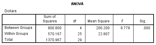
Interpretation:
The most important thing to note in table present here is that SPSS found a significant difference between at least one of the 10 pairs of means. This is shown by the .000 found in the Sig. column. In other words, we now have statistical evidence in support of the researcher’s idea that the expenditures for these trails were not equal. As in the prior tests for differences between means, significance is indicated by the small value (.000) shown in the Sig. column in the table.
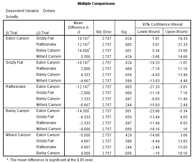
The Scheffe test is another test of significance, but this time the test
compares each possible combination of means one at a time. Examination
of the Scheffe post hoc analysis reveals that there are three mean comparisons that are significantly different. First, we find that there was an average
difference of $10,167 per year on the maintenance of the Eaton Canyon
and Grizzly Flat trails. Second, it is determined that there is an average difference of $12,167 for expenditures on the Eaton Canyon and Rattlesnake
trails. Finally, it is determined that there is an average difference of $14,500
for the Eaton and Bailey Canyon trails. All these differences are statistically
significant at the .05 level.
Summarizing our findings, we may state that the maintenance expenditures for these five mountain trails are significantly different. There is now
statistical support for the researcher’s hypothesis as well as additional details
regarding which of the trail pairs are significantly different.
Continue to Index