Multiple Linear Regression
Multiple linear regression is an extension of simple linear regression in which there is a
single dependent (response) variable (Y) and k independent (predictor) variables Xi
, i = 1,
… , k. In multiple linear regression, the dependent variable is a quantitative variable while
the independent variables may be quantitative or indicator (0, 1) variables. The usual
purpose of a multiple regression analysis is to create a regression equation for predicting
the dependent variable from a group of independent variables. Desired outcomes of such
an analysis may include the following:
1. Screen independent variables to determine which ones are good predictors and thus
find the most effective (and efficient) prediction model.
2. Obtain estimates of individual coefficients in the model to understand the predictive
role of the individual independent variables used.
Appropriate Applications for Multiple Regression Analysis
Design Considerations for Multiple Regression Analysis
A Theoretical Multiple Regression Equation Exists That Describes the Relationship Between the Dependent Variable and the Independent Variables
As in the case of simple linear regression, the multiple regression equation calculated from
the data is a sample-based version of a theoretical equation describing the relationship
between the k independent variables and the dependent variable Y. The theoretical
equation is of the form
Y = α + β1X1 + β2X2 +… + βkXk+ ε
where α is the intercept term and βi
is the regression coefficient corresponding to the ith
independent variable. Also, as in simple linear regression, ε is an error term with zero
mean and constant variance. Note that if βi = 0, then in this setting, the ith independent
variable is not useful in predicting the dependent variable.
The Observed Multiple Regression Equation Is Calculated From the Data Based on the Least Squares Principle
The multiple regression equation that is obtained from the data for predicting the
dependent variable from the k independent variables is given by
Ŷ = a+b1X1+b2X2…+bkXk
As in the case of simple linear regression, the coefficients a, b1
, b2
, … , and bk are least
squares estimates of the corresponding coefficients in the theoretical model. That is, as in
the case of simple linear regression, the least squares estimates a and b1
, … , bk are the
values for which the sum-of-squared differences between the observed y values and the
predicted y values are minimized.
Several Assumptions Are Involved
1. Normality. The population of Y values for each combination of independent variables
is normally distributed.
2. Equal variances. The populations in Assumption 1 all have the same variance.
3. Independence. The dependent variables used in the computation of the regression
equation are not correlated. This typically means that each observed y value must be
from a separate subject or entity.
Hypotheses for a Multiple Linear Regression Analysis
In multiple regression analysis, the usual procedure for determining whether the ith
independent variable contributes to the prediction of the dependent variable is to test the
following hypotheses:
H0
: βi = 0
Ha
: βi ≠ 0
for i = 1, … , k. Each of these tests is performed using a t-test. There will be k of these
tests (one for each independent variable), and most statistical packages report the
corresponding t-statistics and p-values. Note that if there were no linear relationship
whatsoever between the dependent variable and the independent variables, then all of the
βis would be zero. Most programs also report an F-test in an analysis of variance output
that provides a single test of the following hypotheses:
H0
: β1 = β2 =…= βk = 0 (there is no linear relationship between the dependent
variable and the collection of independent variables).
Ha
: At least one of the βis is nonzero (there is a linear relationship between the
dependent variable and at least one of the independent variables).
The analysis-of-variance framework breaks up the total variability in the dependent
variable (as measured by the total sum of squares) by that which can be explained by the
regression using X1
, X2
, … , Xk
(the regression sum of squares) and that which cannot be
explained by the regression (the error sum of squares). It is good practice to check the pvalue associated with this overall F-test as the first step in the testing procedure. Then, if
this p-value is less than 0.05, you would reject the null hypothesis of no linear relationship
and proceed to examine the results of the t-tests. However, if the p-value for the F-test is
greater than 0.05, then you have no evidence of any relationship between the dependent
variable and any of the independent variables, so you should not examine the individual ttests. Any findings of significance at this point would be questionable.
Hypothetical Example
Click Here To Download Sample Dataset (SPSS Format)
Research Scenario and Test Selection
The researcher wants to understand how certain physical factors may affect
an individual’s weight. The research scenario centers on the belief that an
individual’s “height” and “age” (independent variables) are related to the individual’s “weight” (dependent variable). Another way of stating the scenario is
that age and height influence the weight of an individual. When attempting
to select the analytic approach, an important consideration is the level of
measurement. As with single regression, the dependent variable must be
measured at the scale level (interval or ratio). The independent variables are
almost always continuous, although there are methods to accommodate discrete variables. In the example presented above, all data are measured at the
scale level. What type of statistical analysis would you suggest to investigate
the relationship of height and age to a person’s weight?
Regression analysis comes to mind since we are attempting to estimate
(predict) the value of one variable based on the knowledge of the others,
which can be done with a prediction equation. Single regression can be ruled
out since we have two independent variables and one dependent variable.
Let’s consider multiple linear regression as a possible analytic approach.
We must check to see if our variables are approximately normally
distributed. Furthermore, it is required that the relationship between the
variables be approximately linear. And we will also have to check for homoscedasticity, which means that the variances in the dependent variable are
the same for each level of the independent variables. Here’s an example of
homoscedasticity. A distribution of individuals who are 61 inches tall and
aged 41 years would have the same variability in weight as those who are
72 inches tall and aged 31 years. In the sections that follow, some of these
required data characteristics will be examined immediately, others when we
get deeper into the analysis.
Research Question
The basic research question (alternative hypothesis) is whether an individual’s weight is related to that person’s age and height. The null hypothesis is the opposite of the alternative hypothesis: An individual’s weight is
not related to his or her age and height.
Therefore, this research question involves two independent variables,
“height” and “age,” and one dependent variable, weight. The investigator
wishes to determine how height and age, taken together or individually,
might explain the variation in weight. Such information could assist someone attempting to estimate an individual’s weight based on the knowledge
of his or her height and age. Another way of stating the question uses the
concept of prediction and error reduction. How successfully could we predict someone’s weight given that we know his or her age and height? How
much error could be reduced in making the prediction when age and height
are known? One final question: Are the relationships between weight and
each of the two independent variables statistically significant?
Sample Output
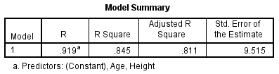
Interpretation:
R column of the table here shows a strong multiple correlation coefficient. It represents the correlation coefficient when both independent variables (“age” and “height”) are taken together and compared with the dependent variable “weight.” The Model Summary indicates that the amount of change in the dependent variable is determined by the two independent variables—not by one as in single regression. From an “interpretation” standpoint, the value in the next column, R Square, is extremely important. The R Square of .845 indicates that 84.5% (.845 × 100) of the variance in an individual’s “weight” (dependent variable) can be explained by both the independent variables, “height” and “age.” It is safe to say that we have a “good” predictor of weight if an individual’s height and age are known
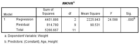
The ANOVA table indicates that the mathematical model (the regression equation) can accurately explain variation in the dependent variable. The value of .000 (which is less than .05) provides evidence that there is a low probability that the variation explained by the model is due to chance. We conclude that changes in the dependent variable result from changes in the independent variables. In this example, changes in height and age resulted in significant changes in weight.
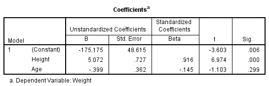
As with single linear regression, the Coefficients table shown in Figure 21.13
provides the essential values for the prediction equation. The prediction equation takes the following form:
Ŷ = a + b1x1 + b2x2,
where Ŷ is the predicted value, a the intercept, b1 the slope for “height,”
x1 the independent variable “height,” b2 the slope for “age,” and x2 the
independent variable “age.”
The equation simply states that you multiply the individual slopes by
the values of the independent variables and then add the products to the
intercept—not too difficult. The slopes and intercepts can be found in the
table shown in Figure 21.13. Look in the column labeled B. The intercept
(the value for a in the above equation) is located in the (Constant) row
and is -175.175. The value below this of 5.072 is the slope for “height,” and
below that is the value of -0.399, the slope for “age.” The values for x are
found in the weight.sav database. Substituting the regression coefficients,
the slope and the intercept, into the equation, we find the following:
Weight = - 175. 175 + (5.072 * Height) − (0.399 * Age).
Further, if we notice p-value for age as a independent variable then, it has no significant relationship with weight as the value is 0.299 which is greater
than alpha value of 0.05. So, we can consider that the Height is only variable which is contributing significantly in explaining the variability of Weight.