Correlation Analysis
A statistic that is often used to measure the strength of a linear association between two variables is the correlation coefficient. Specifically, the correlation covered in this chapter is called Pearson’s correlation coefficient (yes—it’s the same Pearson who measured the fathers and sons). In this section, we refer to Pearson’s correlation coefficient as simply the “correlation coefficient.” The theoretical correlation coefficient is often expressed using the Greek letter rho (ρ) while its estimate from a set of data is usually denoted by r.
Unless otherwise specified, when we say “correlation coefficient,” we mean the estimate
(r) calculated from the data. The correlation coefficient is always between −1 and +1,
where −1 indicates that the points in the scatterplot of the two variables all lie on a line
that has negative slope (a perfect negative correlation), and a correlation coefficient of +1
indicates that the points all lie on a line that has positive slope (a perfect positive
correlation). In general, a positive correlation between two variables indicates that as one
of the variables increases, the other variable also tends to increase. If the correlation
coefficient is negative, then as one variable increases, the other variable tends to decrease
and vice versa. (Neither of these conditions implies causality.)
A correlation coefficient close to +1 (or −1) indicates a strong linear relationship (i.e., that
the points in the scatterplot are closely packed around a line). However, the closer a
correlation coefficient gets to 0, the weaker the linear relationship and the more scattered
the swarm of points in the graph. Most statistics packages quote a t-statistic along with the
correlation coefficient for purposes of testing whether the correlation coefficient is
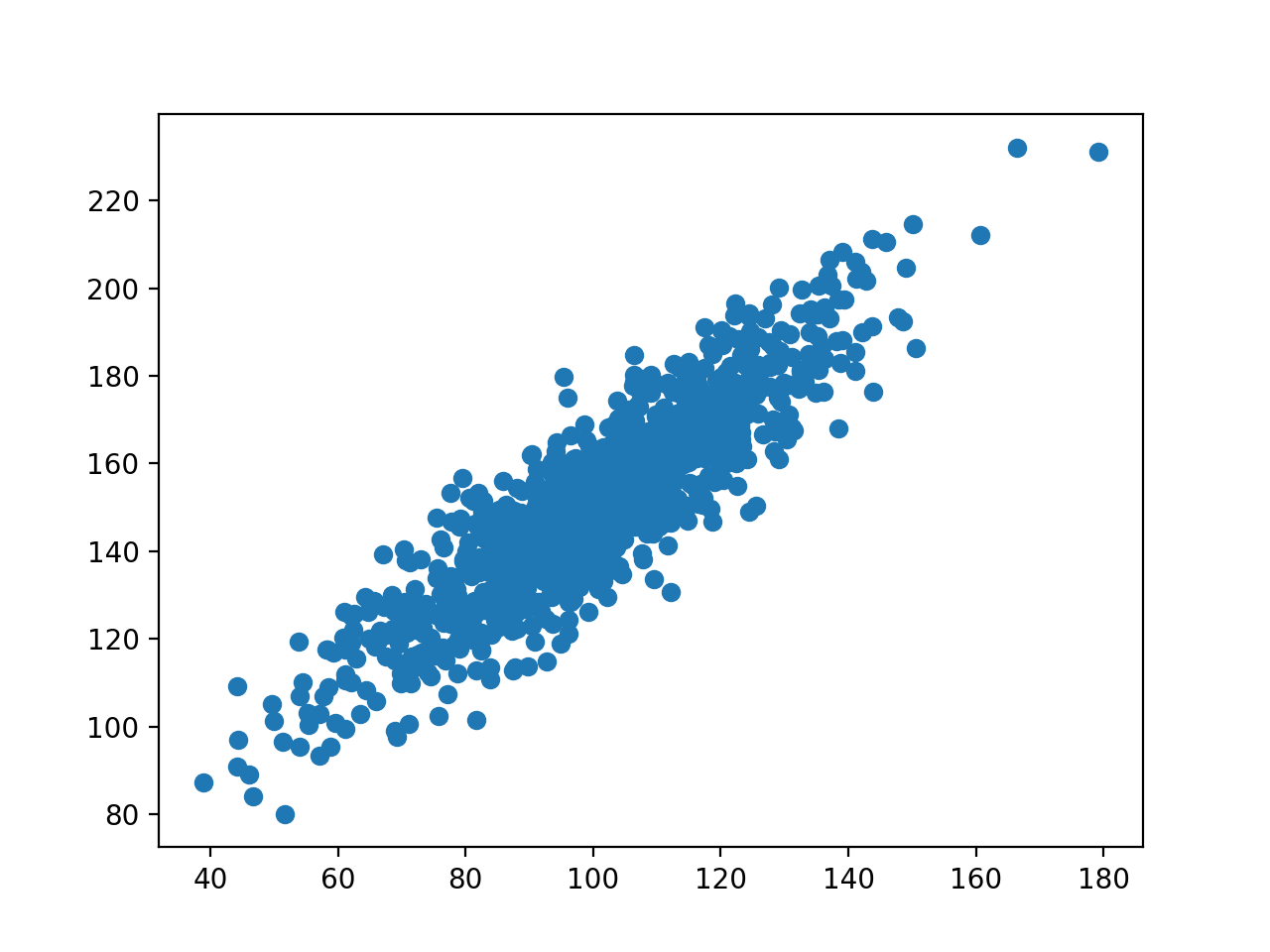
significantly different from zero. A scatterplot is a very useful tool for viewing the
relationship and determining whether a relationship is indeed linear in nature.
Appropriate Applications for Correlation Analysis
The correlation coefficient might be used to determine whether there is a linear relationship between the following pairs of variables:
Design Considerations for Correlation Analysis
1. The correlation coefficient measures the strength of a linear relationship between the
two variables. That is, the relationship between the two variables measures how
closely the two points in a scatterplot (X-Y plot) of the two variables cluster about a
straight line. If two variables are related but the relationship is not linear, then the
correlation coefficient may not be able to detect a relationship.
2. Observations should be quantitative (numeric) variables. The correlation coefficient
is not appropriate for qualitative (categorical) variables, even if they are numerically
coded. In addition, tests of significance of the correlation coefficient assume that the
two variables are approximately normally distributed.
3. The pairs of data are independently collected. Whereas, for example, in a one-sample
t-test, we make the assumption that the observations represent a random sample from
some population, in correlation analysis, we assume that observed pairs of data
represent a random sample from some bivariate population.
Hypotheses for Correlation Analysis
The usual hypotheses for testing the statistical significance of a Pearson’s correlation
coefficient are the following:
H0
: ρ = 0 (there is no linear relationship between the two variables).
Ha
: ρ ≠ 0 (there is a linear relationship between the two variables).
These hypotheses can also be one-sided when appropriate. This null hypothesis is tested in
statistical programs using a test statistic based on Student’s t. If the p-value for the test is
sufficiently small, then you reject the null hypothesis and conclude that ρ is not 0. A
researcher will then have to make a professional judgment to determine whether the
observed association has “practical” significance. A correlation coefficient of r = 0.25 may
be statistically significant (i.e., we have statistical evidence that it is nonzero), but it may
be of no practical importance if that level of association is not of interest to the researcher.
Effect size (discussed below) addresses this issue.
Tips and Caveats for Correlation Analysis
One-Sided Tests
The two-sided p-values for tests about a correlation reported by most statistics programs can be divided by two for one-sided tests if the calculated correlation coefficient has the same sign as that specified in the alternative hypothesis.
Variables Don’t Have to Be on the Same Scale
The correlation coefficient is unitless. For example, you can correlate height (inches) with weight (pounds). In addition, given a set of data on heights and weights, it does not matter whether you measure height in inches, centimeters, feet, and so on and weight in pounds, kilograms, and so on. In all cases, the resulting correlation coefficient will be the same.
Correlation Does Not Imply Cause and Effect
A conclusion of cause and effect is often improperly inferred based on the finding of a significant correlation. It is important to understand that correlation does not imply causation. Causation is difficult to imply (let alone prove) and is a task fraught with many problems.
The Effect Size Provides a Description of a Correlation’s Strength
The effect size for a correlation measures the strength of the relationship. For correlation, r
serves as the numeric measure of the effect size whose strength can be interpreted
according to criteria developed by Cohen (1988):
When r is greater than 0.10 and less than 0.30, the effect size is “small.”
When r is greater than 0.30 and less than 0.50, the effect size is “medium.”
When r is greater than 0.50 the effect size is “large.”
Effect sizes smaller than 0.10 would be considered trivial. These terms (small, medium,
and large) associated with the size of the correlation are intended to provide you with a
specific word you can use to describe the strength of the correlation in a write-up.
Correlations Provide an Incomplete Picture of the Relationship
Suppose, for example, that you have found that for first-year students at a certain university, there is a very strong positive correlation between grades (from 0–100) in rhetoric and statistics. Simply stated, this finding would lead one to believe that rhetoric and statistics grades are very similar (i.e., that a student’s score in rhetoric will be very close to his or her score in statistics). However, you should realize that you would get a strong positive correlation if the statistics grade for each student tended to be about 20 points lower than his or her rhetoric grade. (We’re not claiming that this is the case—it’s just a hypothetical example!) For this reason, when reporting a correlation between two variables, it is good practice to not simply report a correlation but also to report the mean and standard deviation of each of the variables. In addition, a scatterplot provides useful information that should be given in addition to the simple reporting of a correlation.
Hypothetical Example
Click Here To Download Sample Dataset (SPSS Format)
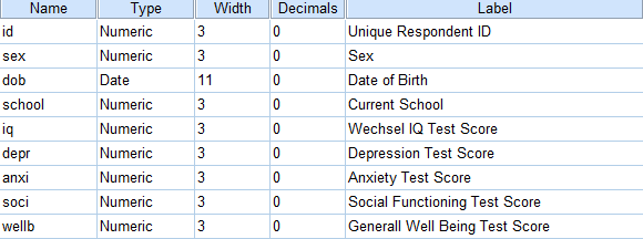
We'll use adolescents.zip, a data file which holds psychological test data on 128 children between 12 and 14 years old. Part of its variable view is shown below.
Sample Output
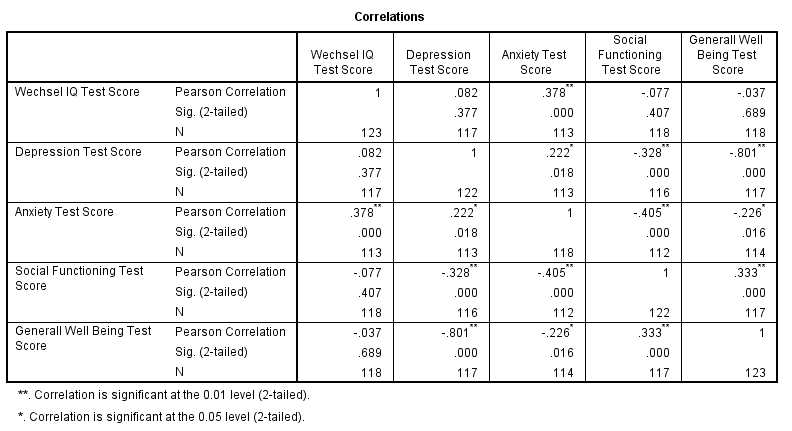
Interpretation:
Now let's take a close look at our results: the strongest correlation is between depression and overall well being : r = -0.801. It's based on N = 117 children and its 2-tailed significance, p = 0.000. This means there's a 0.000 probability of finding this sample correlation -or a larger one- if the actual population correlation is zero.
Note that IQ does not correlate with anything except for Anxiety Test Score. Its strongest correlation is 0.378 at Sig level of 0.01 with anxiety and p = 0.000 so it's only statistically significant.
Continue to Index